User Tools

Site Tools


en:ecovirt:roteiro:metap_uma:metap_chuvarcmdr

Metapopulations and propagule rain - Tutorial in EcoVirtual

 Ênio and Beto walkin in the rain http://desenhos.kids.sapo.pt/a-chuva.htm

In this exercise, we will simulate the dynamics of a metapopulation in which the probabilities of local extinction and patch colonization by our virtual species are constant - the model called propagule rain. In this model, there is a constant source of migrants that can colonize any empty patch, and that's where the model name comes from.

In this model, the variation of the fraction of occupied patches in time is described by the following equation:

$$\frac{df}{dt} = I - E $$

here, I is the migrant entry rate, and E the exit rate. From this, we can define a simple model for the dynamics of the patch occupancy of the metapopulation:

$$\frac{df}{dt} = p_i(1 - f)- p_e f $$

here, $p_i$ is the probability of immigration or colonization, $p_e$ is the probability of extinction, and f is the fraction of occupied patches (number of occupied patches / total number of patches). These are the parameters of our model.

Besides it is mathematically the most simple model,it was described more recently in comparison with ohter metapopulation methods that we will present 1). An important feature of this model is that it is not closed, making it biologically more complex.

Equilibrium

Our simple mode, described above, allow us to calculate a very important trait of the system : the equilibrium solution. The equilibrium here is related to the stability of occupied patches in time, defined by:

$$\frac{df}{dt} = 0$$

With little of algebra, we can calculate the fraction of occupied patches in equilibrium:

$$\hat{f} = \frac{p_i}{p_i + p_e} $$

We could go further and analyse the stability of this equilibrium, but we will only assume that this equilibrium is stable. See the tutorial about stability for the definitions of kinds of stability.

Simulatin Metapopulations

Let's imagine a scenario in which a virtual landscape has a certain number of habitat patches that can be either empty or occupied by our species. Just to make things easier, we will represent this landscape having a certain number of columns and rows ($n_{col}=20$ and $n_{row}=20$), totalizing 400 patches. Let's define the occupancy proportion at the initial time step as $f = 0.25$ (or 100 occupied patches). Our virtual species has an immigration probability of 10% ($p_i= 0.1$) and an extinction probability of 5% ($p_e=0.05$).

Questions

So far, we know that this landscape has a certain capability of accommodating the species, defined by the number of available patches, and that 1/4 of this patches is occupied at the moment. We also know that the colonization probability is larger than the patch extinction probability. Our question is: what is the long term behavior of this population, in this landscape, assuming that all environmental conditions remain the same?

Iterating

The game we will play is like we had a board with 400 tiles, representing our landscape, with 100 of them initially occupied by our pieces. Every turn, for each tile, we are drawing a random number from 1 to 100 (a super sized die with 100 sides!). If the patch is occupied, and the number we get is between 1 and 5, (0.05 probability), we take that piece from the board. If the tile is empty and the number is between 1 and 10 (0.10 probability), we put a new piece there. If none of this conditions trigger, we just leave the tile as it were.

Now, we just need to do this several times and observe at each time step what happened, annotating the proportion of occupied patches (which is out variable of interest).

Using EcoVirtual

As running a board with 400 tiles by hand would be boring and take a long time, we will use EcoVirtual to run the game for us.

To proceed, you must have the R environment with the Rcmdr and Ecovirtual packages installed and loaded. If you do not have and do not know how to have them, see the Installation page.

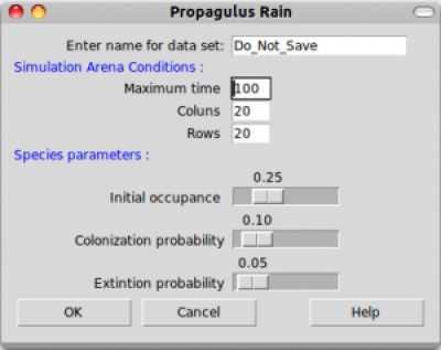
Caso tenha seguido as instruções da página de instalação, partindo da premissa que as instruções funcionam, terá na tela a janela do Rcmdr aberta e uma opção de menu EcoVirtual. Clique nesse menu e depois em Metapopulation em seguida em Seed Rain…. A seguinte janela de opções deve se abrir:

seedrain.png

The parameters of the function are:

Option Parameter Definição
data set name of the R object in which to save the simulation
Maximum time $tmax$ number of iterations
columns $cl$ number of habitat columns in our landscape
rows $rw$ number of habitat rows in our landscape
initial occupancy $f0$ fraction of patches occupied when the simulation begins
colonization probability $pi$ Colonization probability
extinction probability $pe$ Extinction Probability

Run some simulations to understand how the model parameters affect the trajectory and final result (equilibrium) for the population. Below, there are some suggestions of parameter combinations:

Simultion$tmax$$cl$$rw$$f0$$pi$$pe$
1 100 20 20 0,2 0,5 0,2
2 100 20 20 0,2 0,5 0,5
3 100 20 20 0,05 0,2 0,8
4 100 20 20 0,05 0,050,8
5 100 20 20 0,10 0,05 0,9
6 100 10 10 0,05 0,05 0,5
7 100 5 5 0,10 0,05 0,95
8 100 20 20 0,01 0,05 0,95
9 100 5 5 0,01 0,9 0,99
10 100 20 20 0,9 0,9 0,99
11 100 5 5 0,01 0,1 0,99

Next questions

Now it's up to you! Try to answer the following questions:

  • when you run the function several times with the same parameters, do the results stay the same? Why?2)
  • What happens with the variation of the occupancy fraction over time when:
    • the number of patches is very large? Or very small?
  • the probabilities of colonization and extinction are very large?
  • or very small?
  • what about when the initial fraction is very different fr the equilibrium $F=\frac{p_i}{p_i-p_e}$? 3)
  • What conditions lead to population extinction in this model?
Tips
  • To answer the questions above, you need to compare the results of several simulations. You can save the graphs you have generated by right-clicking the graph window.
  • Notice that there are two graphs being shown, one shows the status of the landscape in four time steps, and the other shows the variation of patch occupancy over time. One can hide the other, so move the windows so you can see them all.
  • The graphical windows are not closed between the simulations. From time to time, save those you are interested in and close the others.
  • If you have skills in R programming and are interested in the functions code, take a look at the propagule rain R tutorial

To learn more

  • Gotelli, N. 2007. Ecologia. Londrina, Ed. Planta. Capítulo 4.
  • Stevens, M. H. 2009. A primer of ecology with R. New York. Springer.Capítulo 4.
  • Gotelli, N. 1991. Metapopulation models: the rescue effect, the propagule rain, and the core-satellite hypothesis. The American Naturalist, 138: 768-776. pdf no site do autor
1)
This model was described by Nicholas Gotelli in 1991, see the reference in the end of the tutorial
2)
you should understand this in order to answer the next questions
3)
For details on this formula, take a look at the chapter 4 of Gotelli, 2007
en/ecovirt/roteiro/metap_uma/metap_chuvarcmdr.txt · Last modified: 2017/10/10 17:56 by melina.leite