−Table of Contents
Density-independent population dynamics - Tutorial in EcoVirtual
A population in which birth rates and mortality are constant has a growth or decrease independently of its own density. This situation is usually related to the lack of constraint on growth when resources are unlimited, but can also be associated with the extinction of populations.
Discrete time
Growth rate
Let's imagine now a population with constant growth and mortality rates and without migration. The population grows or is observed at regular intervals. The population size in the next time step (Nt+1) is the number of individuals of the previous generation (Nt) plus the number of births (B), and less the number of deaths (D) in the time interval:
Nt+1=Nt+B−D
The numbers of deaths and births are the result of per capita rates multiplied by population size:
B=bNt D=dNt
where: b = per capita birth rate at each generation; d = per capita death rate at each generation. Note that the rate does not change with the size of the population, and the number of births and deaths is proportional to the population size. Let's just clarify one more premise, for educational purposes: births and deaths occur simultaneously in the population at the time interval t. We can then say that:
Nt+1=Nt+bNt−dNt Nt+1=Nt+(b−d)Nt
if we define a factor of discrete growth: rt=b−d
Nt+1=(1+rt)Nt Nt+1Nt=1+rt
As 1+rt is a constant, let's designate it as λ, a positive number that expresses the proportional increase of the population from one generation to another. Therefore:
λ=Nt+1Nt⟹Nt+1=λNt
Projection of the population in discrete time
We can then project our population in every t time step. For example:
If a population with 100 individuals has a per capita birth rate of 0.8/yr and a mortality rate of 0.75/yr, which is the expected size of the population in the next year?
Nt+1=100×(1+0,8−0,75)=100×1,05=105
We can also project the population for other generations, using iterations: Nt+2=105×1,05=110,25 Nt+3=110,25×1,05=115,7625
continuing and taking the population size at zero time (N0):
Nt+4=N0×λ×λ×λ×λ Nt+4=N0λ4
Generalizing:
Nt=N0λt
So, for our example, the projection for 10 time intervals is
100×1,0510=162,8895
Continuous time
With a little algebraic manipulation, the equation for discrete time
Nt+1 = (1+rt)Nt
Can be rewritten as
Nt+1−Nt = ΔN = rtNt
which explains that the growth rate ΔN=Nt+1−Nt is proportional to the population size Nt. This is an essential characteristic of population growth without limits at a constant rate:
Omni vivo ex vivo 1)
The speed of growth is the variation in the number of individuals ΔN divided by the time this change has been made, Δt. In discrete time model Δt=1, by definition. It is an interval which can be as large as a generation. This makes sense if the population size changes occur in discrete intervals, for example in semelparous species with synchronized breeding season.
However, the population sizes of most species vary continuously. Differential calculus was created to describe this kind of dynamic. Since the problem is that changes can occur at any time, the key concept here is the instantaneous rate, or derivative.
Instantaneous growth rate
If births and deaths can happen all the time, it makes more sense to think in an instantaneous speed of the population size. This equates to reducing Δt so much that it can be considered an instant. This instantaneous velocity is the derivative of the population size, that we represent with dN/dt, to differentiate from the speed at large intervals and arbitrary ΔN/Δt 2).
Now we can express that the instantaneous velocity of a population is proportional to the population size with the equation:
dNdt=rN
This is the continuous time constant rate population growth model. The parameter r is called instantaneous growth rate per capita. This rate r expresses the average number of offspring that each individual of the population produces in a very short time interval. Because of that, many ecology books indicate that the unit of r is individuals / (individual * time). Physicists and mathematicians are more stringent and remember that the correct expression of the unit is 1 / time.
Projection of the population in continuous time
To predict the size of a population that grows at a constant rate in continuous time we use the equation
N(t)=N0ert
And the relation between the instantaneous growth rate and the growth rate of the discrete model is
r = ln(λ)
Why? Why? Why?
Simulating density-independent growth
To proceed, you must have the R environment with the Rcmdr and Ecovirtual packages installed and loaded. If you do not have and do not know how to have them, see the Installation page.
Let's use EcoVirtual to predict the size of populations that grow at constant rates without limit in continuous and discrete time.
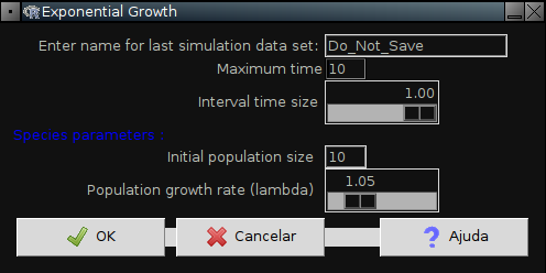
In the Rcmdr window, click on the menu option EcoVirtual, and then click on One population. Then, on Exponential growth. Two windows will open, one with options like this
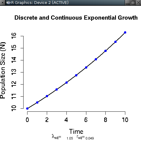
and another with a chart like this:
Arrange the windows so that the graph is always visible, even when you change values in the options window.
Parameters
The parameters of our density-independent function are:
| Option | parameter |
|---|---|
Enter name for last simulation data set | R object |
Maximum time | tmax |
Interval time size | intt |
Initial population size | N0 |
Population growth rate (lambda) | lambda |
What's in the chart?
It shows the population size versus time predicted by the model. The blue dots indicate the population sizes predicted by the growth model in discrete time
Nt=N0λt
using the values of N0 and λ from the options window. The black line indicates the population sizes predicted by the growth model in continuous time
N(t)=N0ert
using the same values from the options window. To do this, the λ from the options window is used to calculate the corresponding instantaneous per capita growth rate of the continuous model by the relation:
r=ln(λ)
The values for the discrete model are dots, because this model predicts the size of the population at discrete intervals. The continuous time model, however, forecasts the size of the population at any time, and that’s why it is represented by a continuous line.
The dots overlap the line because EcoVirtual uses equivalent growth rates to make comparable projections. Below the X-axis of the graph are the values of λ and r used in the simulation.
Exercises: playing in the fields of the Lord
 In his memorable lessons on population dynamics, physicist Roberto Kraenkel usually says he does not know if Heaven exists, but if it does, he knows that only there populations grow without limits. Nevertheless, he continues, the models for this type of growth are essential to understand the dynamics of real population, as well as Newton's unrealistic first law is essential to understand the movement of bodies in space.
So let's use EcoVirtual to explore the behavior of growth models at constant rates!
Varying the rate of growth
Try different values of the discrete growth rate λ with the option Population growth rate (lambda) from the options window. This will also change the continuous growth rate r. See the effect on the graph and use a calculator to check the correspondence between the two rates, indicated below the x-axis of the graph.
Question
At what value or range of values for λ and r the population: - increases ? - decreases? - remains stable ?
Varying the interval in the discrete model
The option Interval time size defines a new time interval for the discrete time model. The new interval value is a fraction of the original value of one. So, if you choose 0.5 for this option, the projections of the discrete model are recalculated for intervals corresponding to half of the original range. Therefore, you will see blue dots on the graph every half unit of time. Changing the interval to 0.25 you’ll have projections for intervals that are a quarter of the original unit, and there will be dots on the graph for every 0.25 unit of time.
Notice that as you decrease the discrete model time interval, the dots get closer, until they seem to form a continuous line. In other words, the projection at discrete intervals tends to the projection in continuous time as the intervals are reduced!
In fact, the exponential model can be seen as a limit of the discrete model. Details are in the already indicated script rates, derivatives and the exponential function. But for this to work, EcoVirtual recalculates the value of λ and the corresponding value for r for each new range of discrete time. And here's our question: how are these calculations made? More precisely:
Question
Given a rate of discrete growth for a time interval of value of a unit,
λ1=Nt+1Nt
how to calculate the growth rate for a fractional interval
λ1/n=Nt+1/nNt
so that by the end of a unit of time the growth rate remains λ1? Check your solution against the values that EcoVirtual returns when you reduce the discrete time interval by half (Interval time size=0.5 option).
Two tips
- Another way of thinking about the problem is to remember that the discrete growth in an original unity of time in the unit rate is λ1 and in the fractional rate is λn1/n. The solution of the problem is to make these two amounts equal.
Extra exercise : grow up BRAZIL
This exercise uses population survey from IBGE to model and predict brazilian population growth . First, download the dataset:
To follow the tutorial in the wiki:
To open the exercise directly in your computer (offline):
- censo.zip, unzip and open the .html file in your browser.
To learn more
- Gotelli, N. J. 2007. Ecologia. Planta, Londrina. Chapter 1 is a very didactic introduction to growth models without dependence on density.
- Population dynamics from first principles. Chapter 2 from Complex Population Dynamics. Peter Turchin, Princeton Univ Press, 2003. This thought-provoking text argues that the exponential growth model is for Biology what Newton's laws are for Physics.
- Vandermeer, J. 2010. How Populations Grow: The Exponential and Logistic Equations Nature Education Knowledge 3(10):15. Another very didactic text, with considerations of the environmental consequences of human population growth..


