−Table of Contents
Population dynamics with density dependende - Tutorial in EcoVirtual
 The population growth model with constant growth rate may leave the impression that its predictions are useless. As a matter of fact, we never see in nature a population that exhibits an exponential growth for very long. The tutorials for these models show that bacteria, for example, can grow in an exponential manner for some time, until…
This limitation of the exponential growth (i.e., the “until…”) is related to the model assumptions. In this cases, the assumption that the conditions and resources that each individual experiences are constant in time.
This assumption is very unrealistic - but not more unrealistic than the assumptions of the Newton's law of inertia. In nature, there are no bodies that keep moving in a stable motion with the same speed and direction forever. Anyway, this law helps us to understand our world, and together with Newton's other laws it helps us predict the trajectories of planets with a reasonable precision.
In the same way that a miniature car stops moving some time after being propelled because of attrition (between its own pieces, and between the wheels and the ground), a population slows down its growth until it stops. That happens due to several factors, even if it has a theoretical potential to keep on growing in exponential fashion.
Density effects
A change in the density of a population can have effects on the vital rates of the individuals. For example, in social animals for which cooperation increases survival, an increase in density may increase the survival probability (Allee effect).
The marmots (those cute little rodents!) live in groups where there are guards to alert about the present of predators (birds of prey - which are less cute). These guard shifts reduce the per capita predation in the population. The positive effects of density in a population, although seem to be very evolutionarily beneficial, have evolved in few linages of organisms1).
On the other hand, the negative effects of density dependence are universal. Even for those species that present cooperation, at some point in increasing density, the negative effects overrides the positive.

Why are the negative effects of density so widespread? A simple reason: to exist means to occupy a space. Space is a finite resource - even if renewable - and two bodies may not occupy the same space2). Another simple reason: the individuals from a same population need “exactly” the same resources. Even if the resources are abundant, if the population grows too much, it will become limiting. We call these kind of interaction between individuals from a population intra-specific competition3), the simplest form of population size self-regulation.
The logistic model
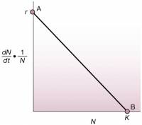
A simple way to think about the density effect in a population is to make the population growth and the population size to have a negative linear relation. We only need to take care to see that we're modeling each individual (per capita) effect in the population growth rate. See the following graph:
This graph depicts the contribution of each individual (1N ) to the growth rate of the entire population dNdt as a function of the total number of individuals (N). The maximum growth rate is r 4) and the maximum size of the population is K: the support capacity.
We can write down the equation for this first-order function, y=a+bx, where a is the intercept and b the inclination coefficient:
dNdt1N=r−rKN
With a little bit of algebra…
dNdt1N=r(1−NK)
dNdt=rN(1−NK)
We can interpret this equation in the following way: the growth speed, dN/dt, grows near an exponential rN when N is small - because the expression (1−NK) is near unity. On the other hand, when the population size gets near the support capacity K, the expression (1−NK) tends to zero, and so does the growth speed. We can think of the expression (1−NK) as the unused portion of the support capacity.
There is an analytical solution for the equation above, that can be expressed as a population size as a function of time5). It can be written as:
Nt=K1+((K−N0)/N0)e−rt
What is the take-home message?!
The most important thing to notice in our model is the linear dependence of density. The biological interpretation is way easier in the differential equation formulationdNdt=rN(1−NK).
It's also important to know that this differential equation has an analytical solution, which allows us to figure out easily the population size for each value of time.
Simulating the logistic model
To proceed, you must have the R environment with the Rcmdr and Ecovirtual packages installed and loaded. If you do not have and do not know how to have them, see the Installation page.
Let's now use EcoVirtual to simulate different populations with density dependence and try to interpret their possible biological meaning.
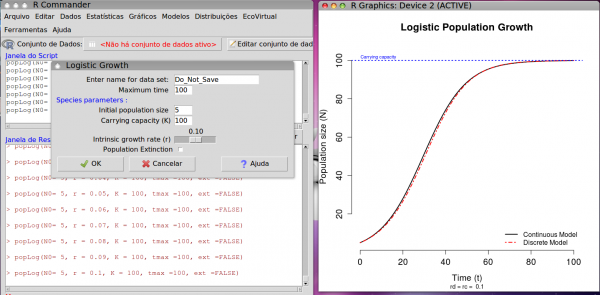
On the EcoVirtual menu, open the window Logistic Growth, from the One Population menu:
The parameters of the function are:
| Option | parameter |
|---|---|
| maximum time | tmax |
| Initial population size | N0 |
| Carrying capacity | K |
| intrinsic growth rate | r |
| population extinction | ext=TRUE |
Questions
- The logistic curve is often referred to as S-shaped. Does the graph on the window have this shape? Change the parameters and try to find the hidden S shape. Which parameter makes the S more evident? Why?
- Make simulations to confirm the following statement: “the final population is the same, independently of the initial condition (N0)”. Use r=0.05 and K=100, and values for N0 below and above the carrying capacity.
- Make simulations to confirm the following statement: “when a population is disturbed from its equilibrium, it takes longer to stabilize if its number is increased than if its number is decreased”. Run your simulations for r values between 0.01 and 1.0 and K=100.
Discrete time models
The graph from EcoVirtual shows two logistic models which are executed with the same parameters: (1) continuous time and (2) discrete time. Although the continuous model's growth rate is an instantaneous rate (rc) while the discrete model's is a rate of individuals by time interval6), the models are, up a a certain point, equivalent. The discrete coefficient rd can be written as:
rd=λ−1
with: λ=Nt+1Nt
Damped oscillations
The discrete time model has a very distinct behavior for very high population growth rates. Let's slowly increase this parameter and see:
- simulate populations with growth rates ranging from 1.0 up to 1.8 and describe the difference between the discrete and continuous time simulations.
- change the maximum time to 107) and propose an explanation for the discrete time model.
Limit cycles and...
What happens with the discrete model projections if we increase the growth rate even more? Simulate populations with rates equal to 2.2 and 2.5 and see for yourself. Use long maximum times to see whether the population stabilizes, and shorter times to see what's happening on a better resolution.
Questions
- Is there a regularity for this values of growth rate?
- What is the difference between the models?
Now simulate a population for growth rate of 2.9 and answer:
- Is there any regularity in this projection?
- Is the trajectory reversible?
- Do changes in the population initial size affect the trajectory?
Bifurcation map
 Apparently simple non-linear functions may exhibit this unusual behavior of generating unpredictable patterns. Actually, there is a lot of regularity in the seeming disorder of these functions. One constant that was described in this disorder is the ratio between the interval up to a bifurcation and the interval to the next bifurcation8). Few people expected that, 25 centuries after Pythagoras described the constant π, a new universal constant could be discovered.
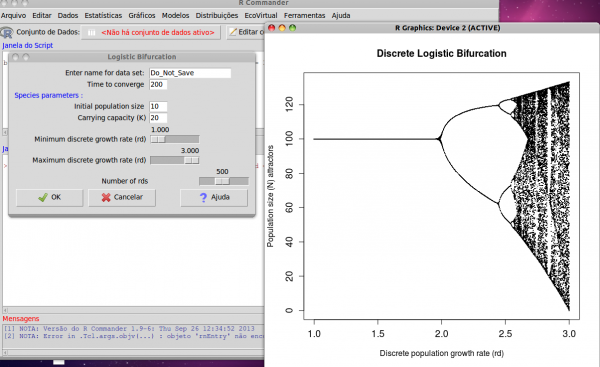
One way to see the behavior of these populations as we change the discrete growth rate rd is by plotting a logistic bifurcation plot. The proposal is to map the stability points (attractors) of the population growth. To do this, we need to simulate populations with several values for rd for some time and store the values for which there's convergence. However, we need to let these simulations run for a while to make sure that, if there is a convergence point, it has been reached.
The function bifAttr* of the EcoVirtual package does this. Its parameters are:
| Option | parameter |
|---|---|
| Time to convergence | tmax |
| Initial population size | N0 |
| Carrying capacity | K |
| Minimum discrete growth rate (rd) | minrd |
| Maximum discrete growth rate (rd) | maxrd |
| Number of rds | nrd |
Let's see this map, using the default values for the function! On the EcoVirtual menu, open the Logistic Bifurcation, on the One Population menu, and click OK**. The following graph should appear:
Atividade
- identifique os padrões de bifurcação;
- varie os parâmetros K e N0 e veja se há modificação no padrão geral do mapa de bifurcação. O que isso significa?
Patterns inside chaos
 Another pattern that we can observe is that chaos windows are intercalated with limit cycles. One more pattern: in the limit cycle windows, there's a modification on the bifurcation rule: it starts on a stable point (K), then starts on 3, 5, 7, 9… and each prime number. That is, the start of the regular period cycles and bifurcation starts with every prime number. Another fascinating pattern is that the patterns repeat on different scales, like fractal dimension objects.
Questions
- where are the starting points of the limit cycle windows with different periods (3, 5, 7…)?
- show the pattern repetition at different scales.
Use small intervals of rd, by changing minrd and maxrd, and look where there are gaps in the bifurcation map.
Exercises
- Assume that one population of butterflies is growing according to the logistic model. If the carrying capacity of an area is 500 butterflies e r=0.1 individuals / (individual * month), what is the maximum possible growth rate for this population?
- Attempting to maximize the fishing yields, a fisheries biologist is trying to keep a stable population of lake trout at 500 individuals. Assuming that the r for the trout is 0.005 individuals / (individual * month), and predict what is the population growth if the population stays at 500 individuals, and what is the population growth if the population is increased in 600 additional individuals.
- Demonstrate that the decline of a population above its carrying capacity is always faster than the corresponding growth for a population below the carrying capacity. Why is it so? (Tip: represent the initial population above or under the carrying capacity as k ± x individuals)
To learn more
- Gotelli, N. J. 2007. Ecologia. Planta, Londrina. O capítulo 2 é uma introdução muito didática aos modelos de crescimento com dependência da densidade.
- Fernandez, F. 2000. Capítudo 5 - Da Falsa Questão de Elton a um mundo novo. In: O Poema Imperfeito. Cronicas de Biologia, Conservação da Natureza e seus Heróis. Editora UFPR, Curitiba. pdf
- Sherratt T. & David M. Wilkinson. 2009. Capítulo 6 - Is Nature Chaotic? In: Big Questions in Ecology and Evolution. Oxford University Press, USA. pdf
- May, R. M. 1976. Simple mathematical models with very complicated dynamics. Nature 261: 459-467. O artigo clássico em que Robert May demonstrou que modelos muito simples de dinâmica populacional podem exibir comportamento caótico.
- Population dynamics from first principles. Capítulo 2 de Complex Population Dynamics. Peter Turchin, Princeton Univ Press, 2003. Este texto instigante apresenta os modelos clássicos de crescimento populacional como leis análogas às da Física. Uma abordagem muito original dos modelos e sua importância para a teoria ecológica.
- Edwards, W. J. & Edwards, C. T. 2011. Population Limiting Factors. Nature Education Knowledge 3(10):1. Introdução ao conceito de fatores limitantes dependentes e independentes da densidade.
- Vandermeer, J. 2010. How Populations Grow: The Exponential and Logistic Equations. Nature Education Knowledge 3(10):15. Outro texto muito didático, com considerações sobre as consequências ambientais do crescimento populacional humano.
- Introduction to dynamic systems and chaos, excelente curso online do site Complexity Explorer.
![[[http://en.wikipedia.org/wiki/Marmot]] [[http://en.wikipedia.org/wiki/Marmot]]](/lib/exe/fetch.php?w=150&tok=0e45fb&media=http%3A%2F%2Fupload.wikimedia.org%2Fwikipedia%2Fcommons%2Fthumb%2F3%2F3b%2FMarmot-edit1.jpg%2F320px-Marmot-edit1.jpg)


