Introduction to multivariate ordination

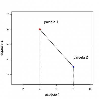
Ordination refers to a series of techniques that are used to transform multivariate data, in order to present them in few dimensions (generally two to three), with a minimal loss of information. This example shows a graphical representation of two parcels in a dimensional space of two species.

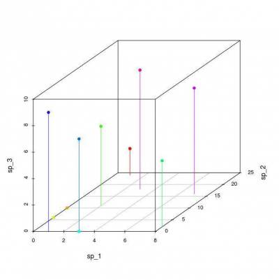
When we have only two attribute dimensions (in our case, two species), the graphical representation of the objects is straightforward. With three dimensions we are still able to represent our parcels in one graph, but increasing the dimension makes the graphical representation impossible.

The several methods for ordination, such as Principal Component Analysis (PCA), Correspondence Analysis (CA) or Non-Metric Multidimensional Scaling (NMDS), have been proposed to reduce the number of dimensions of data to allow visualizing the relationships between objects.

> ls()
[1] "dev"  "mea"  "samp.cont"  "samp.disc"  

The polar ordination was one of the first methods to be developed, and it was widely used due to its simplicity. Although it was superseded by later (and more sophisticated methods), the polar ordination is relevant for the biological interpretation of its results. Moreover, understanding this simple algorithm will help to understand the shared logic behind more complex techniques.

The objective here is to represent the parcels in a system of coordinates in a manner such that the distance between the parcels represent the similarity between them, what may reveal the underlying environmental gradient. Here, we will use the original algorithm developed by Bray and Curtis (1957) to study plant community data. To start our analysis, we first calculate the Bray-Curtis dissimilarity between the parcels¹⁾.

The following function calculates the Bray-Curtis dissimilarity between each pair of parcels. Copy and paste it in your R session:

dis.bc<-function(data){
  nplot=dim(data)[2]
  similar=matrix(NA,ncol=nplot,nrow=nplot)
  rownames(similar)<-paste("plot", c(1:nplot))
  colnames(similar)<-paste("plot", c(1:nplot))
  for(i in 1:(nplot-1)){
    m=i+1
    for(m in m:nplot){
      bc.dist=sum(
          abs(data[,i]-data[,m]))/(sum (data[,c(i,m)])
          )
          similar[m,i]=similar[i,m]=bc.dist
          diag(similar)<-0
    }
  }
  return(round(similar,3))          
}

• 1. Use the function above to generate the dissimilarity matrix for our sample of a community:

dis1.cont=dis.bc(amost.cont)

• 2. Calculate, for each parcel, the sum of the dissimilarities between itself and all other parcels:

sumdist1.cont=apply(dis1.cont, 1, sum, na.rm=TRUE)
sumdist1.cont
<code>

  * **3.** Mark the parcel with the greater sum of dissimilarities((that is, the parcel that is least like the others)) and store its value to mark the start of our x axis (which we will call **ax**):

<code>
max(sumdist1.cont)
names.parc = names(sumdist1.cont)
parc.ax = names.parc[sumdist1.cont==max(sumdist1.cont)][1]
parc.ax

• 4. Find now the parcel that is least similar to this first parcel. This will mark our second reference in the x axis (which we will call bx):

dist.ax=dis1.cont[,parc.ax]
dist.ax
max.ax=max(dist.ax)
max.ax
parc.bx=names.parc[dist.ax==max.ax]
parc.bx

• 4a. It may happen that more than one parcel is tied as being the least similar to ax. In this case, we use the largest sum of distances to other parcels as a tiebreaker:

somamax.bx=max(sumdist1.cont[parc.bx])
parc.bx=parc.bx[sumdist1.cont[parc.bx]==somamax.bx][1]
parc.bx

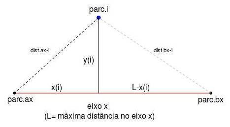
• 5. Now that we have two references on the x axis, ax and bx, we can calculate the position of each parcel in this axis AND in the orthogonal axis as well. This works like the triangulation used in telemetry: by placing two receptors in known points and measuring the distance from the emitter (one animal with a radio-collar, for example) to both receptors, it is possible to determine the two-dimensional coordinates where the animal is. Look in the following schema:

To do this, we use Beal's equation (Beal, 1965), which is nothing more than solving together for the hypotenuse of the triangles above. After some algebra, Beal equation can be written as:

$$ x_i \ = \ \frac{ L^2 \ + \ dist_{ax_i}^2 \ - \ dist_{bx_i}^2 }{2L} $$

where “L” is the length of the x axis (or the dissimilarity between parc.ax and parc.bx, “dist_{ax_i}” is the dissimilarity between parcel “i” and parc.ax, and “dist_{bx_i}” is the dissimilarity between parcel “i” and parc.bx. Check out the notation in the figure above.

• 5a. Now that we understood Beal's equation, we need to organize our values for the distance of all parcels in relation to our reference points parc.ax and parc.bx. We have the values for parc.ax stored in the dist.ax object, which we will examine below. Then, we will store the values for parc.bx in a new object called dist.bx:

dist.ax
dist.bx=dis1.cont[,parc.bx]
dist.bx

• 5b. Now apply Beal's equation to all parcels to find their position in the x axis:

xi = (max.ax^2 + dist.ax^2 - dist.bx^2)/(2*max.ax)
xi

• 6. Finally, we can find their position in our second axis using Pythagoras theorem:

$$ y_i = \sqrt{dist_{ax_i}^2 - x_i^2} $$

yi=sqrt((dist.ax)^2-xi^2)
yi

• 6a. At last, we adjust parc.bx in the y axis:

yi[parc.bx]=max.ax
yi

• 7. We now have all the coordinates of all our parcels in two coordinate axis! Let's organize them

in a single object and plot it:

op1.cont=data.frame(xi,yi)
op1.cont
plot(op1.cont, pch=19, col=rainbow(length(xi)), xlab="x axis", ylab="y axis")
text(op1.cont+0.01, labels=rownames(op1.cont))

We are such cool guys that we have organized a single function that does all the above steps, so you won't have to follow them again for new data. See below:

ordena.polar=function(dist)
{
  sumdist1.cont=apply(dist, 1, sum, na.rm=TRUE) + apply(dist,2,sum, na.rm=TRUE)
    nomes.parc=names(sumdist1.cont)
    parc.ax=nomes.parc[sumdist1.cont==max(sumdist1.cont)][1]
    dist.ax=dist[,parc.ax]
    max.ax=max(dist.ax)
    parc.bx=nomes.parc[dist.ax==max.ax]
    if(length(parc.bx)>1)
    {
      somamax.bx=max(sumdist1.cont[parc.bx])
        parc.bx=nomes.parc[sumdist1.cont==somamax.bx][1]
        parc.bx
    }
  dist.bx=dist[,parc.bx]
    xi= (max.ax^2 + dist.ax^2 - dist.bx^2)/(2*max.ax)
    yi=sqrt((dist.ax)^2-xi^2)
    yi[parc.bx]=max(dist.ax)
    op.xy=data.frame(xi,yi)
    opx=jitter(op.xy[,1],10)
    opy=jitter(op.xy[,2],10)
    plot(opx, opy, pch=19, col=rainbow(length(xi)), xlim=c(-0.1, 1.1), ylim=c(-0.1,1.1), main="Polar ordination", sub="Bray-Curtis Dissimilarity")
    text(opx-0.02,opy-0.02 , labels=paste("p",1:dim(dist)[1], sep=""), cex=0.7)
    return(op.xy)
}

We will apply this function to the continuous community data to check if it's working properly:

ordena.polar(dis1.cont)

Now, we will apply it for the discrete virtual community as well. First, remember to use the disc.bc function to create a dissimilarity matrix:

dis1.disc=dis.bc(amost.disc)

Then, simply run the ordena.polar in this new matrix:

ordena.polar(dis1.disc)

What is the interpretation of the patterns you have found? Remember how each community was created.

Some tips for interpreting results of ordination data, not only of Polar Ordination but applicable to other analyses as well. It's based on material produced by Michael Palmer on his great site on ordination:

1. The direction of the axes is arbitrary and should not affect interpretation;
2. The numerical scale of the axes is not very useful for the interpretation (there are some exceptions such as DCA, where the scale is in beta units diversity);
3. In the PO, as well as many other ordination techniques, the order of the axes is important. Thus, the x axis is more important for the interpretation of the environmental gradients than the y axis;
4. Previous experience of the studied system and knowledge of the relevant literature are the most powerful tools for the interpretation of underlying gradient patterns revealed by ordination;
5. The interpretation of the axes in addition to the first two (when the analysis produces them) is possible and the decision of where to stop is an arbitrary question, depending on the quantity and quality of data. In some techniques, there are statistics that help to make this decision;
6. It is desirable that the axes are not correlated, which is secured by some techniques. Thus it is possible to interpret the axes as different gradients.

After going through the steps to build virtual communities, sample them and apply classification and sorting methods, we believe that you understand the basic principles of analytical methods used for the description of communities in ecology. As stated earlier in these tutorials, there are many different methods to know and many things still to research in relation to these methods. A vast and interesting world!

• Ordination Methods for Ecologists, Mike Palmer. (an excellent panorama on the ordination techniques and their use in ecology).
• Clustering and Classification methods for Biologists: site from the course by Alan Fielding.
• Manly, B. 2008. Métodos Estatísticos Multivariados: Uma Introdução. 3 Ed. Artmed, Porto Alegre. (One of the best introductions to multivariate techniques for biologists).
• Prado, P.I. et al. 2002. Ordenação multivariada na ecologia e seu uso em ciências ambientais. Ambiente & Sociedade, (10), 69-83.
• Valentin, J. 2012. Ecologia Numérica: Uma Introdução à Análise Multivariada de Dados Ecológicos. Interciência, Rio de Janeiro. (Another good introductory text)
• Legendre, P., & Legendre, L. 2012. Numerical ecology. Elsevier, Amsterdan. (The complete reference for numerical ecology. Very didactic, although it's a more advanced reference).