−Table of Contents
Successional niche
Usually the competition between species is viewed as a “all or nothing” instantaneous process. However, observing nature we realize that plants with high capacity for colonization generally have high metabolic rates (respiration, photosynthesis and allocation of reproductive tissue). These high rates allow for the plants to grow and reproduce more quickly, which may give them an extra advantage in competitive interaction. Imagine a forest where a clearing was opened by a fallen tree and both species, the best competitor and the better disperser reach it at the same time. In this situation, imagining that the best competitor will immediately remove the other does not seem very reasonable, simply because there is no resource limitation yet. On the other hand, the species that have the highest growth rate can reproduce before the resource limitation occurs and it is driven to local extinction by competition.
Pacala and Rees model
This period, before the environmental resource reduction, creates an ephemeral niche that was called by Pacala and Rees (1998) the “succession niche”. These authors developed a simple model to test their ideas. They have established five possible states in the system:
- Vacant: none of the species
- Early: occupied only by the species of early succession
- Susceptible: occupied by the late species, but susceptible to initial invasion because the resources are still abundant
- Mixed: occupied by both species, on the road to competitive exclusion
- Resistant: occupied only by the late species and resistant to invasion
Given these states the succession process can have several possible trajectories:
- VACANT → EARLY → MIXED → RESISTANT
- VACANT → SUSCEPTIBLE → MIXED → RESISTANT
- VACANT → SUSCEPTIBLE → RESISTANT
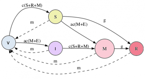
Let's create our model. For simplicity, rather than we model each species, we model the state and its transitions in a similar way that we model the states of individuals in a population: remember the matrix models of Leslie and Lefkovich from the earlier classes?! Look at the diagram below to understand the state transitions:
This model has four parameters: c, α, m and γ:
- c is the base colonization rate
- α is the early species relative colonization rate
- m is the death or disturbance rate
- γ is the rate of competitive exclusion
With these four parameters, we can model the variation of the proportion of states over time, with the expressions that appear in the transitions from the figure above. Solid lines indicate increase in proportion and broken lines decreases in proportion. For example, variation in the SUSCEPTIBLE state is given by:
(dS)/dt = [c(S + R + M)]V - [αc(M+E)]S - gS - mS
Using EcoVirtual
The following parameters can be changed:
| option | parameter | effect |
|---|---|---|
| data set | R object | stores the simulation results |
| Simulation Arena Condition | Basic simulation parameters | |
| Maximum time | tmax | number of model iterations to be run |
| columns | cl | number of columns in the habitat |
| rows | rw | number of rows in the habitat |
| Initial Stages Proportions | Initial state | |
| Early Stage | er | fraction of patches initially occupied by sp2 |
| Susceptible | /sc | fraction of patches initially with sp1, and that may be invaded by sp2 |
| Mixed | mx | fraction of patches initially with both species |
| Resistant | rs | fraction of patches initially with sp1, and that may not be colonized sp2 |
| Colonization rates | Colonization parameters | |
| Better competitor | c1 | sp1 colonization coefficient |
| Poor competitor | c2 | sp2 colonization coefficient |
| General Parameters | General parameters | |
| Competitive exclusion | ec | probability of transition from SC and MX to RS |
| Disturbance | dst | proportion of patches that is kept empty |
Testing with a high rate of competitive exclusion and low disturbance:
tmax=50,
rw=100,
cl=100,
c1=0.2,
c2=0.8,
ec=0.5,
dst=0.04,
er=0.08,
sc=0.02,
mx=0,
rs=0,
Now, let's simulate some scenarios to see what happens:
- Reduce the competitive exclusion to 0.1.
- Keep ec in 0.1 and increase the disturbance to 0.1 as well.
- Put both species with the same colonization rate (c1=0.4 and c2=0.4).
What is the biological interpretation for your results? Connect your answer to:
- ecological succession
- successional niche
- intermediate disturbance
- competition
Questions
- Write a short essay in which you provide an interpretation for all of the scenarios above, and connect the trajectories to the concepts of:
- ecological succession
- successional niche
- intermediate disturbance
- competition
- How can you change the function used to create a scenario in which you would only study the tradeoff between colonization vs. competition? Explain your answer.
- Is coexistence possible if you only consider the effect of the successional niche? Use a simulation to justify your answer.
To learn more
- Pacala, S. & M. Rees. 1998. Models suggesting field experiments to test two hypotheses explaining successional diversity. The American Naturalist 152(2): 729:737.
- Stevens, M.H.H. (2009) A primer in ecology with R. New York, Springer. capítulo 9

