−Table of Contents
Stability in Dynamical Systems - Tutorial in R
Equilibrium and stability are very important concepts in ecology, but they have many conflicting definitions. One of the most used was brought from the branch of physics and mathematics called dynamical systems analysis.
It is this approach that brought to ecology equations to describe the dynamics of populations, such as logistic growth equation and the system of Lotka-Volterra equations.
There are techniques designed to evaluate whether these systems of equations have equilibrium points, and, if so, whether these equilibriums are stable. Robert May (1972) used these tools to demonstrate a somewhat surprising result: the stability in food webs decreases with the increase of species and complexity.
Preparation: the R environment
This exercise will be done using R (R Core Team 2012), but you don't need to know the R language, because we will provide the commands ready to be executed. They are printed in this page, but also on the annex script. The only thing you need to know is how to run these commands on R. You can either copy and paste them in the R command line, or use the script file. Just follow these steps:
- Install the R environment in your computer, along with the libraries
deSolveandrootSolve. The
offical R page has some instructions, but you can also read our R installation tutorial.
- Create a new folder to place your exercises.
- Copy to this folder the following files:
- Open R and the script file
eq_comandos.r. Make sure that your working directory is where it the files are. - The commands in the script are in the same order as they are presented in this tutorial. Follow the tutorial, sending the commands as they are required.
- If you're not sure how to send the commands, follow this tutorial.
- Load in your R session the packages and functions that we will use in this tutorial:
library(deSolve)
library(rootSolve)
source("eq_funcoes.r")
One population
Let's start with the stability analysis from the well-known logistic population growth equation:
V = rN (1−NK)
Here V is the population growth speed1), r is the intrinsic population growth rate, and K is the carrying capacity.
We can plot the graph for the logistic population growth for any value of parameters using R, with the function plota.logist:
plota.logist(n=2,r=0.1,K=50,time=200)
The arguments for this function are:
n: initial population sizer: intrinsic population growth rateK: carrying capacitytime: maximum simulation time
Try changing some parameters and see the results.
Logistic Equilibrium
The basic question for stability analysis in dynamical systems is: where are the system's stable equilibrium points? To answer that, we first need to say what we mean by equilibrium:
dNdt=0
There are two population sizes that satisfy this condition for the logistic equation:
- N = K
- N = 0
The fact that these are equilibrium points has a lot of biological meaning: the population cannot grow when it arrives at the carrying capacity, nor when it's empty.
Make sure that these are really equilibrium points with:
## Starting with N=K
plota.logist(n=50,r=0.1,K=50,time=200)

## Starting with N=0
plota.logist(n=0,r=0.1,K=50,time=200)
Logistic stability
Are these equilibrium points stable? Let's define more precisely what we mean by that:
A small perturbation might be a small increase or decrease in the population size. Our graphing function has some parameters to introduce perturbations:
perturb: amount of perturbationt.perturb: perturbation time
Use these arguments to add one individual2) to the populations starting with population sizes zero and K:
## Perturbation with N=K
plota.logist(n=50,r=0.1,K=50,time=200, perturb=1, t.perturb=100)
## Perturbation with N= 2
plota.logist(n=2,r=0.1,K=50,time=200, perturb=1, t.perturb=100)

## Perturbation with N=0
plota.logist(n=0,r=0.1,K=50,time=50, perturb=1, t.perturb=10)
Questions
- Are this points stable?
- What is the biological interpretation for this?
Mathematical interpretation
The stability criterion we use evaluates the behavior of the growth rate, when the population size varies slightly around the equilibrium point. What is the relationship between growth rate and population size in the logistic equation?
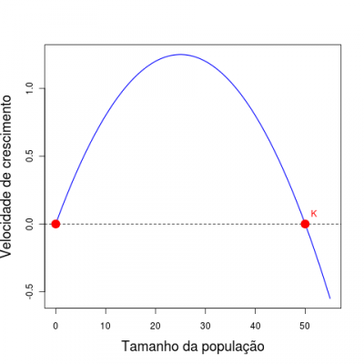
See the figure below: the speed has a quadratic relationship with the population size, forming a parabola. The equilibrium points, wherein the growth velocity is zero, are marked in red 3).
When the population is small, the population growth makes the growth rate increase, ie, more population size accelerates its growth.
From a certain population size, called inflection point of the curve, the increase in the population causes a decreasing speed. From this point on population size “brakes”4) growth.
This is the very expression of the logistic equation: growth close to exponential when the population is small, and reducing speed up to a full stop, when the population reaches the carrying capacity. Therefore, the speed has a positive relationship with population size close to equilibrium N=0. Therefore, a small increase above zero increases the growth rate, which increases the population size, which further increase the growth rate. This is an unstable equilibrium: a small perturbation will make the population size move away from it.
At the point K=N, the opposite happens: the rate has a negative relationship with population size. If we reduce the population slightly below K, it will grow, but this growth will reduce the growth rate until the rate is zero. If we increase the population slightly above the carrying capacity, the speed is negative 5), and the population will reduce back to K, as the negative speed also slows down. Thus, disturbances in the neighborhood of the carrying capacity are attracted back to this point.
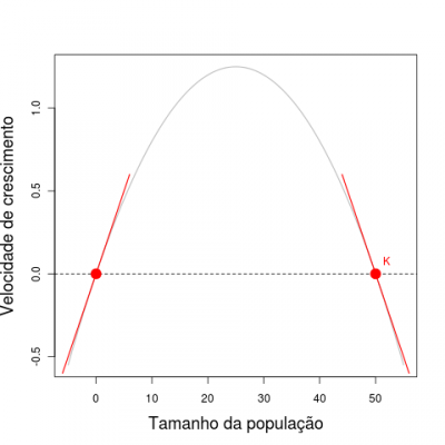
In summary, what defines the stability around an equilibrium point is the sign of the relationship between the growth rate and population size in this neighborhood. This corresponds to the sign of the slope of a line tangent to the equilibrium point, which is the derivative of velocity with respect to population size at these points.
Below is the same parable of the previous figure, now with tangent lines added to the equilibrium points. The slope of the line is positive at the point N=0 and negative at the point N=K.
With this, we arrive at a criterion of local stability for one population with continuous growth:
In mathematical terms, this is:
dVdN|ˆN < 0
We can read this as: “The derivative of V in respect to N at the point ˆN is negative”.
Why so many bold words? To remember that all this reasoning is valid only in the neighborhood of a point.
The derivative can be seen as a straight line approximating a function at one point. In the neighborhood of this point this linear approach works well, and we can focus on evaluating the behavior of the tangent line slope (ie, the sign of the derivative at point) in order to represent small changes to the function.
So the full name of what is presented in this tutorial should be local stability analysis by linear approximation.
It evaluates the response of systems of differential equations after small disturbances in the neighborhood of their equilibrium points. This is done under the premise that in this neighborhood the speed functions are well approximated by its derivatives.
This analysis does not provide any guarantee on the outcome of major disruption, and may also fail to systems with strongly nonlinear behavior.
To learn more
- Gotelli, N. 2007. Ecologia. Londrina, Ed. Planta. (A basic reference about the dynamic models in ecology).
- May, R.M. 1972. Will a large complex system be stable? Nature, 238, 413-414. (The classic paper that established the concept of trophic network stability as a solution for a Lotka-Volterra system.)
- May, R.M. 2001. Stability and complexity in model ecosystems. Princeton, Princeton University Press. (In this influent monograph, Robert May develops the ideas of the 1972 paper. The first edition is from 1973, but it was republished by Princeton Landmarks of Biology in 2001.)
- Sarah P. Otto & Troy Day 2007. A Biologist's Guide to Mathematical Modeling in Ecology and Evolution. Princeton, Princeton University Press. (A great introduction to the maths behind these models, from biologists to biologists, using more intuitive approaches to the problems. A great source if you want to understand the details of the analyses used in this tutorial. See also the book site.)
- Our tutorial on Stability and diversity, in which the analysis done here is generalized for a system with more than one species.
- R Development Core Team (2012). R: A language and environment for statistical computing. R Foundation for Statistical Computing, Vienna, Austria. ISBN 3-900051-07-0, URL http://www.R-project.org/.


